Application Exercise 3e: Demand and Supply
1) Using the Excel programme or in your workbooks, plot the above figures onto a demand and supply graph/ diagram. Ensure that you label the vertical and horizontal axis and the scale is accurate (i.e. ensure that the price and quantity intervals are the same distance apart)
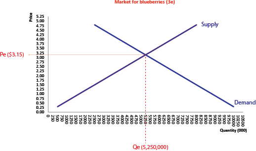
2) Determine the likely equilibrium price and quantity and indicate this on the diagram with Pe and Qe.
The likely equilibrium price is $3.15 and equilibrium quantity is 5,250,000 blueberries.
3) Explain why the blueberry market is in disequilibrium if the price is set at $4.20 per kg and highlight the surplus or shortage on the diagram.
If the price is at $4.20 the market is in disequilibrium because consumers are only willing to demand 3,500,000 blueberries when farmers will supply the market with 7,000,000. This means that the market will be in excess supply (or surplus).

When the market is in excess supply, illustrated by the difference between Q1D and Q1S below (i.e. 3,500,000 blueberries). Too many blueberries will remain unsold and suppliers will eventually reduce price in order to attract demand (an expansion along the demand curve from point 1 to 2 below).
4. Use the diagram to illustrate how the market returns to equilibrium over time, from the disequilibrium in question 3, highlighting the movements along the curves (contraction/expansion) when the price changes.
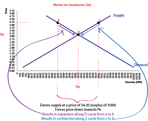
When the market is in excess supply, illustrated by the difference between Q1D and Q1S below (i.e. 3,500,000 blueberries). Too many blueberries will remain unsold and suppliers will eventually reduce price in order to attract demand (an expansion along the demand curve from point a to b below). Over time, profit maximizing producers will also reduce their supply to the market in response to lower prices (a contraction along the supply curve from points c to b). Price will continue to fall in the market for blueberries, resulting in the excess supply getting smaller and smaller until eventually the price will ‘rest’ at the equilibrium price of $3.15. Note that it is possible for producers to reduce the price below the equilibrium price (i.e. they will overshoot equilibrium). In this case, price will eventually rise towards equilibrium as the market will be in a state of excess demand (see next question)
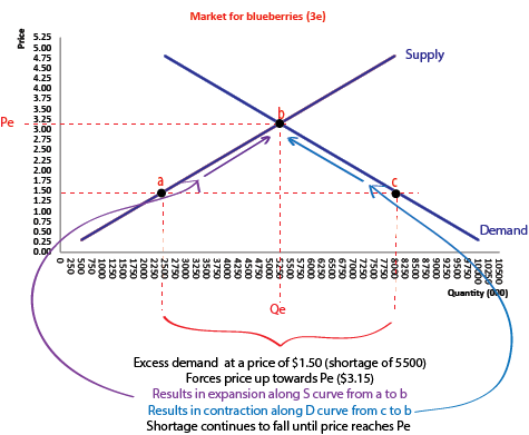
5. Explain why the blueberry market is in disequilibrium if the price is set at $1.50 per kg and highlight the surplus or shortage on the diagram.
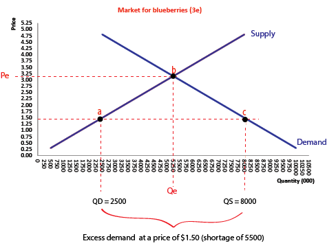
When the market is in excess demand, illustrated by the difference between Q1D and Q1S below (i.e. excess demand of 5,500,000 blueberries). Suppliers will quickly run out of blueberry stocks and seize the opportunity to raise prices. The higher price will work to:
- Reduce consumer demand for blueberries (a contraction along the D curve)
- Increase producers’ willingness to supply over time as higher prices, ceteris paribus, equates to higher profits (an expansion along the supply curve)
Price will continue to rise in the market for blueberries, resulting in the shortage getting smaller and smaller until eventually the price will ‘rest’ at the equilibrium price of $3.15. Note that it is possible for producers to increase the price above the equilibrium price (i.e. they will overshoot equilibrium). In this case, price will eventually fall back towards equilibrium in response to the excess supply.
- Use the diagram to illustrate how the market returns to equilibrium over time from the disequilibrium in question 5, highlighting the movements along the curves (contraction/expansion) when the price changes.